// Interactive Blog Image Analysis & Computer Vision · 2026

Fitting Geometry to Messy Point Clouds

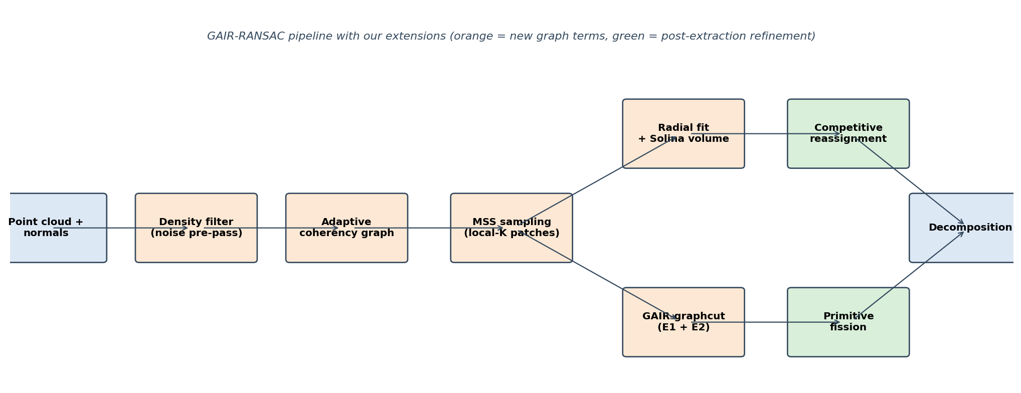
Real depth sensors return noisy, cluttered clouds of 3D points. This project turns those clouds into a handful of clean geometric solids — superquadrics — even when the data is sharp-edged, overlapping, or 30% outliers. We extend the GAIR-RANSAC framework (STAG 2025) with six targeted changes that make it robust enough for real meshes and sensor data.

Authors Miguel Gutierrez · Matteo Paoli · Jasmin Spinetto
Advisors Prof. Luca Magri · Prof. Vincenzo Caglioti
Institution Politecnico di Milano — Image Analysis and Computer Vision

↻ Try the 3D demo GitHub repo GAIR-RANSAC (STAG 2025)

01 — Interactive · real fitted data

Drag to explore the actual results

Everything below is real data from the project — measured point clouds rendered as dots, with the recovered superquadric surfaces overlaid. Drag to rotate, scroll to zoom, right-drag to pan. Switch scenes and layers with the controls.

drag · scroll · right-drag to pan

3D viewer needs WebGL + internet (loads three.js from CDN). The result images further down show the same fits.

02 — The problem

Why superquadrics, and why it's hard

A superquadric is a single implicit equation with 11 parameters that can morph between spheres, ellipsoids, cubes, octahedra, cylinders and bipyramids. That makes it a compact, expressive vocabulary for describing the parts of an object — perfect for robotics, reverse engineering and scene understanding, where you want "three boxes and a cylinder", not a million raw points.

The catch is robustness. Real RealSense and Thingi10K data carry noise, outliers and overlapping structures. Plain least-squares fitting collapses: a single primitive stretches to swallow the whole scene, or sharp corners get rounded off. The GAIR-RANSAC framework casts inlier selection as a graph-cut labelling problem and solves it globally — but it was tuned for smooth, clean shapes. We push it into the hard regime.

Problem formulation

Given an unordered set of noisy 3D points $\mathcal{D}=\{\mathbf{x}_1,\dots,\mathbf{x}_n\}$, the goal is to recover a collection of primitives $\{\theta_1,\dots,\theta_\kappa\}$ that explains the scene. Each primitive is a superquadric, defined implicitly in its canonical frame by the inside–outside function

(1) $$ F(\mathbf{x}_c,\Lambda)=\left[\left(\frac{x_c}{a_1}\right)^{\tfrac{2}{\varepsilon_2}}+\left(\frac{y_c}{a_2}\right)^{\tfrac{2}{\varepsilon_2}}\right]^{\tfrac{\varepsilon_2}{\varepsilon_1}}+\left(\frac{z_c}{a_3}\right)^{\tfrac{2}{\varepsilon_1}}=1, $$

where $\Lambda=\{a_1,a_2,a_3,\varepsilon_1,\varepsilon_2\}$ collects the scale $(a_i)$ and shape $(\varepsilon_1,\varepsilon_2)$ parameters. A rigid transform $T(\Gamma)$ with rotation and translation $\Gamma$ places the primitive in the world frame, so each model carries 11 parameters, $\theta=\Lambda\cup\Gamma$. A point with $F<1$ lies inside the surface, $F=1$ on it, and $F>1$ outside — the shape exponents $\varepsilon_1,\varepsilon_2$ sweep from ellipsoids $(\varepsilon\!\approx\!1)$ to boxes $(\varepsilon\!\to\!0)$ to pinched bipyramids $(\varepsilon\!>\!1)$.

03 — What we changed

Six improvements over the paper

Each change targets a specific failure mode we observed on real data.

01 · DISTANCE

Radial (Solina) residual

The paper's algebraic residual blows up for sharp shapes (ε < 0.3). Our radial residual cancels that blow-up, widening the admissible range from [0.3, 1.3] to [0.1, 1.9] — so cubes, bricks and octahedra become fittable.

02 · GRAPH

Adaptive normal-coherency cut

The paper breaks every sharp edge, shattering cubes at their corners. We cut an edge only where both sides are locally smooth, and flag contact-face edges — keeping solids intact while still separating touching objects.

03 · SAMPLING

Local-K MSS + PCA pose

Instead of sampling globally, we draw minimal sample sets from a local patch neighbourhood, reject coplanar samples via an SVD check, and seed the pose from PCA. The fit converges in 2–3× fewer iterations.

04 · ENERGY

Hardened pairwise term

A coherency floor and an |F−1| inlier gate close an exploit where a stretched superquadric with a large gradient norm fakes a low residual while badly missing the surface.

05 · REFINE

Competitive Chamfer reassignment

After extraction, every point is reassigned to its nearest primitive surface and the fits are refreshed — correcting the drift that sequential RANSAC accumulates. A fission step splits a primitive that wrongly merged two objects.

06 · OUTLIERS

Density-based pre-filter

Sparse "bridge" points let consensus walk between objects. A simple density filter removes them, so a single ε setting holds from clean data up to 30% noise with no per-scene retuning.

At a glance — paper vs. ours

Component	Paper (GAIR-RANSAC)	Ours
Surface distance	(F−1)/‖∇F‖, unstable when sharp	radial residual (a₁a₂a₃)^1/3(F^ε/2−1)
Admissible ε	[0.3, 1.3] — smooth only	[0.1, 1.9] — sharp + smooth
Volume penalty	—	Solina (a₁a₂a₃)^2/3 anti-needle term
Graph-cut rule	drop any C < τ edge	drop only if smooth on both sides + contact-face filter
MSS sampling	global K patches × 2 pts	local-K patches + SVD validity + PCA pose
Post-refinement	sequential remove-and-fit	competitive Chamfer reassignment + fission
Outlier handling	consensus threshold only	+ density pre-filter

04 — Method · the inner fit

Robust single-primitive fitting

Recovering the 11-parameter model $\theta$ from a noisy patch needs a stable residual, careful sampling, and strict inlier gating. The baseline normalises the algebraic error by the surface gradient,

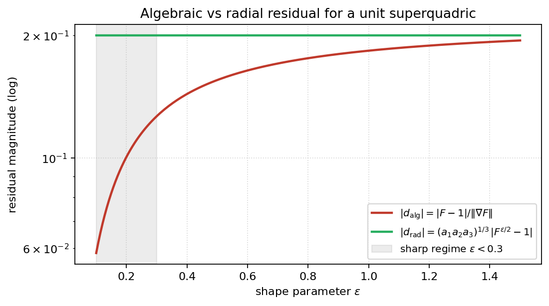
$$ d_{\text{alg}}(\mathbf{p})=\frac{F(\mathbf{p})-1}{\lVert\nabla F(\mathbf{p})\rVert}, $$

which is well-behaved for smooth shapes but blows up as $\varepsilon\to 0$: at a cube edge the gradient vanishes and $d_{\text{alg}}$ becomes unreliable, hiding sharp shapes from the optimiser.

Radial residual + volume penalty

We replace it with the Solina radial residual, which cancels the inner-exponent blow-up and stays well-conditioned across the whole admissible range $\varepsilon\in[0.1,2.0]$:

(2) $$ d_{\text{rad}}(\mathbf{p})=(a_1 a_2 a_3)^{1/3}\left(F(\mathbf{p})^{\varepsilon_1/2}-1\right). $$

To stop the optimiser from trivially driving $d_{\text{rad}}\to 0$ by inflating the scales $a_i$, we add an anti-needle volume penalty $R_{\text{vol}}(\theta)=\lambda_{\text{size}}\,(a_1 a_2 a_3)^{2/3}$, with $\lambda_{\text{size}}=0.05$.

The `|F−1|` inlier gate

A stretched superquadric with a very large $\lVert\nabla F\rVert$ can fake a small $d_{\text{alg}}$ for points physically far from its surface. We close this gradient-driven exploit with a strict second gate on the un-normalised implicit error:

(3) $$ E_1(\mathbf{p})=\begin{cases}\operatorname{err}(\mathbf{p}) & \text{if } |F(\mathbf{p})-1|<\tau_F,\\[2pt] 1 & \text{otherwise,}\end{cases}\qquad \tau_F=0.15. $$

A point is an inlier only if both the spatial distance and the implicit error are small.

Local-K sampling + PCA pose

Standard RANSAC scatters minimal sample sets (MSS) globally, so they routinely straddle two objects. We instead draw each MSS from a single seed patch and its graph neighbours, reject near-coplanar samples with an SVD rank check, and seed the optimiser with a rotation $R_0$ from the PCA of the centred MSS — which converges in 2–3× fewer iterations on elongated shapes.

Adaptive normal-coherency cut

The baseline drops any graph edge whose endpoints have nearly antiparallel normals. That correctly splits a sphere–sphere joint, but it also shatters a single cube: at a corner three faces meet at right angles and the same rule fires. We make the rule adaptive by conditioning on each endpoint's local normal consistency,

(4) $$ c_i=\operatorname*{mean}_{k\in\mathcal{N}(i)}\,\lvert\mathbf{n}_i\cdot\mathbf{n}_k\rvert, $$

close to $1$ in smooth neighbourhoods and well below $1$ near sharp features. An edge $(i,j)$ is cut only when pairwise coherency is low and both endpoints sit in smooth regions:

(5) $$ \text{drop}(i,j)\iff C_{ij}<\tau_C \;\wedge\; c_i>\tilde\tau_C \;\wedge\; c_j>\tilde\tau_C, $$

with $C_{ij}=\tfrac{1}{2}(1+\mathbf{n}_i\cdot\mathbf{n}_j)$, $\tau_C=0.5$, $\tilde\tau_C=0.85$. The cube corner now survives (its own $c_i$ is low) while the sphere–sphere joint is still cut — closing both failure modes at once.

05 — Method · the outer loop

Sequential multi-model extraction

To recover a whole scene $\mathcal{H}=\{\theta_1,\dots,\theta_\kappa\}$, the single-primitive fitter is wrapped in a detect-and-remove loop, with a density pre-filter up front and two global rebalancing steps at the end.

Density-based pre-filter

Sparse outliers form structural "bridges" that merge disjoint objects into one connected component. We score each point by the number of neighbours within radius $r_\rho$,

(6) $$ \rho(\mathbf{p})=\bigl\lvert\{\mathbf{q}\in\mathcal{D}:\lVert\mathbf{p}-\mathbf{q}\rVert

and drop it before graph construction if it lacks support, $\;\rho(\mathbf{p})(7), with \(r_\rho=0.05$ (5% of the bounding-box diagonal) and $k=3$.

Algorithm 1 · Sequential multi-model extraction

in: cloud $\mathcal{D}$, normals $\mathcal{V}$, threshold $\varepsilon$, max models $\kappa$
$\mathcal{D}\leftarrow$ DensityFilter$(\mathcal{D})$
$G_{\text{full}}\leftarrow$ BuildAdaptiveGraph$(\mathcal{D})$; $\mathcal{R}\leftarrow\mathcal{D},\;\mathcal{H}\leftarrow\varnothing$
for $k=1$ to $\kappa$:
$C\leftarrow$ LargestConnectedComponent$(G_{\text{full}}[\mathcal{R}])$
$(\theta_k,I_k)\leftarrow$ ImprovedSingleFit$(\mathcal{D}[C],\mathcal{V}[C],\varepsilon)$
if $\theta_k$ passes Chamfer + Coverage gates: $\mathcal{H}\leftarrow\mathcal{H}\cup\{(\theta_k,I_k)\}$; remove $I_k$ + surface shell from $\mathcal{R}$
$\mathcal{H}\leftarrow$ CompetitiveReassignment$(\mathcal{H},\mathcal{D},\varepsilon)$
$\mathcal{H}\leftarrow$ PrimitiveFission$(\mathcal{H},\mathcal{D})$; return $\mathcal{H}$

Chamfer + coverage gates

A candidate $\theta_k$ fitted on component $C$ with inliers $I_k$ is accepted only if it clears two gates. The Chamfer gate samples $m=1000$ points $S_k$ on the fitted surface and bounds the symmetric squared distance to the data:

(8) $$ \mathrm{CD}(I_k,S_k)=\frac{1}{|I_k|}\sum_{\mathbf{p}\in I_k}\min_{\mathbf{q}\in S_k}\lVert\mathbf{p}-\mathbf{q}\rVert^2+\frac{1}{|S_k|}\sum_{\mathbf{q}\in S_k}\min_{\mathbf{p}\in I_k}\lVert\mathbf{q}-\mathbf{p}\rVert^2\;\le\;\tau_{CD}. $$

The coverage gate rejects locally tight but unrepresentative fits via completeness, $\;|I_k|/|C|\ge\tau_{\text{cov}}=0.7$, and a per-axis axial spread test in the canonical frame $\tilde{\mathbf{p}}=R^\top(\mathbf{p}-\mathbf{t})$:

(9) $$ \frac{\max_p \tilde{p}_i-\min_p \tilde{p}_i}{2a_i}\;\ge\;\tau_{\text{ax}}=0.15,\qquad i\in\{x,y,z\}. $$

Competitive reassignment + fission

Sequential extraction is greedy: early models over-claim points or merge two touching objects into a "mixture fit". Two global post-steps fix this. Competitive reassignment re-labels every point to the nearest fitted surface (within $\varepsilon$) and refits each primitive on its rebalanced inlier set:

$$ \text{label}(\mathbf{p})=\arg\min_{k}\;\min_{\mathbf{y}\in S(\theta_k)}\lVert\mathbf{p}-\mathbf{y}\rVert^2,\qquad \text{s.t. } \lVert\mathbf{p}-\mathbf{y}\rVert\le\varepsilon. $$

Primitive fission then 2-means–clusters each primitive's inliers and splits a suspected mixture-fit when both a bimodal-centre test and a spatial-gap test hold:

(10) $$ \frac{\lVert\mathbf{c}_1-\mathbf{c}_2\rVert}{\max(\sigma_1,\sigma_2)}>\beta_{\text{cent}},\qquad \min_{\mathbf{p}\in I_1,\,\mathbf{q}\in I_2}\lVert\mathbf{p}-\mathbf{q}\rVert>\beta_{\text{gap}}\,\varepsilon, $$

with centroids $\mathbf{c}_1,\mathbf{c}_2$, principal spreads $\sigma_1,\sigma_2$, and $\beta_{\text{cent}}=2.5$, $\beta_{\text{gap}}=3.0$.

06 — Results

From synthetic stress tests to real meshes

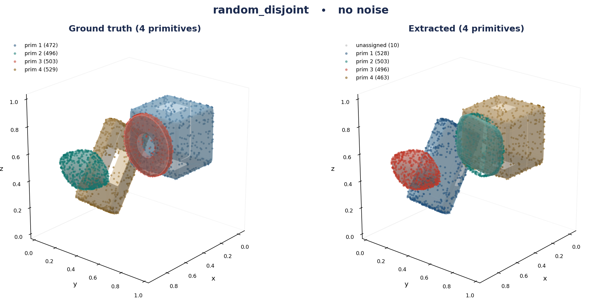
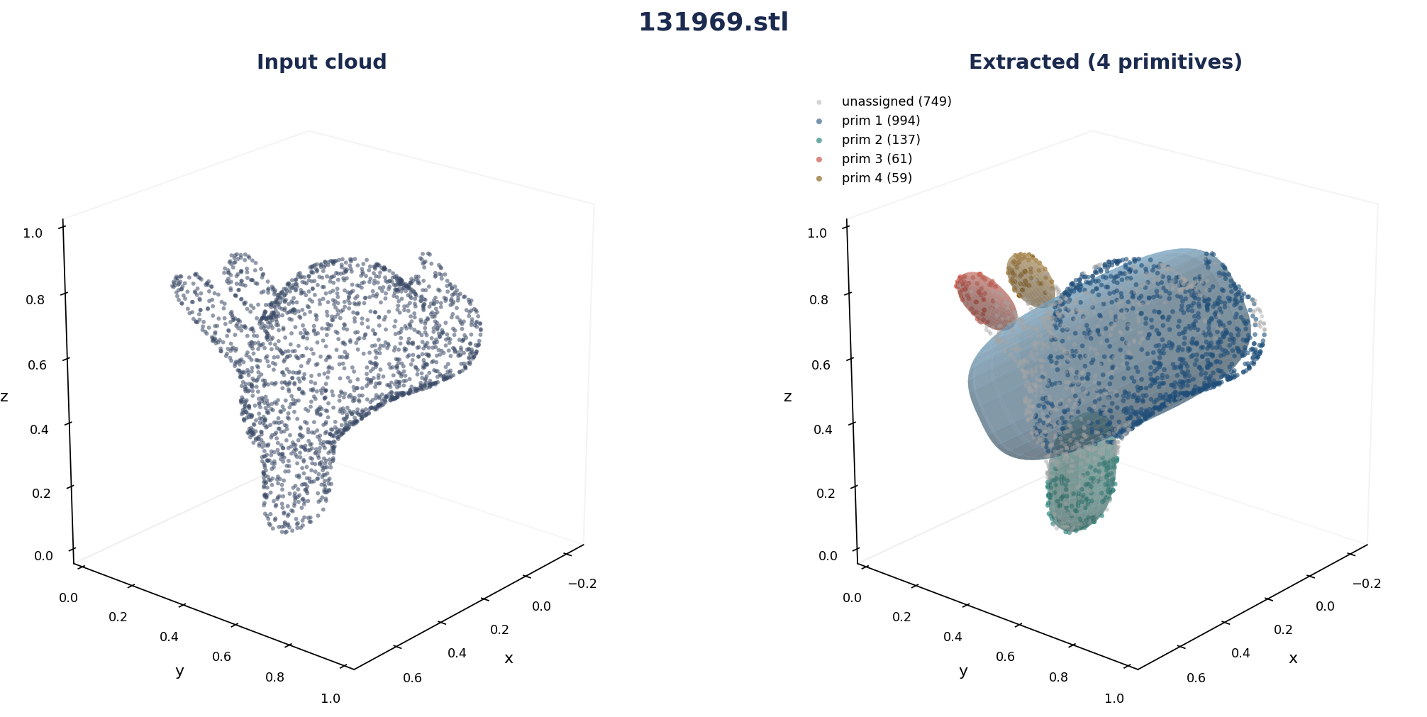
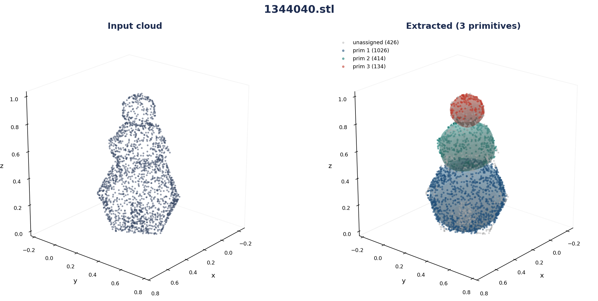
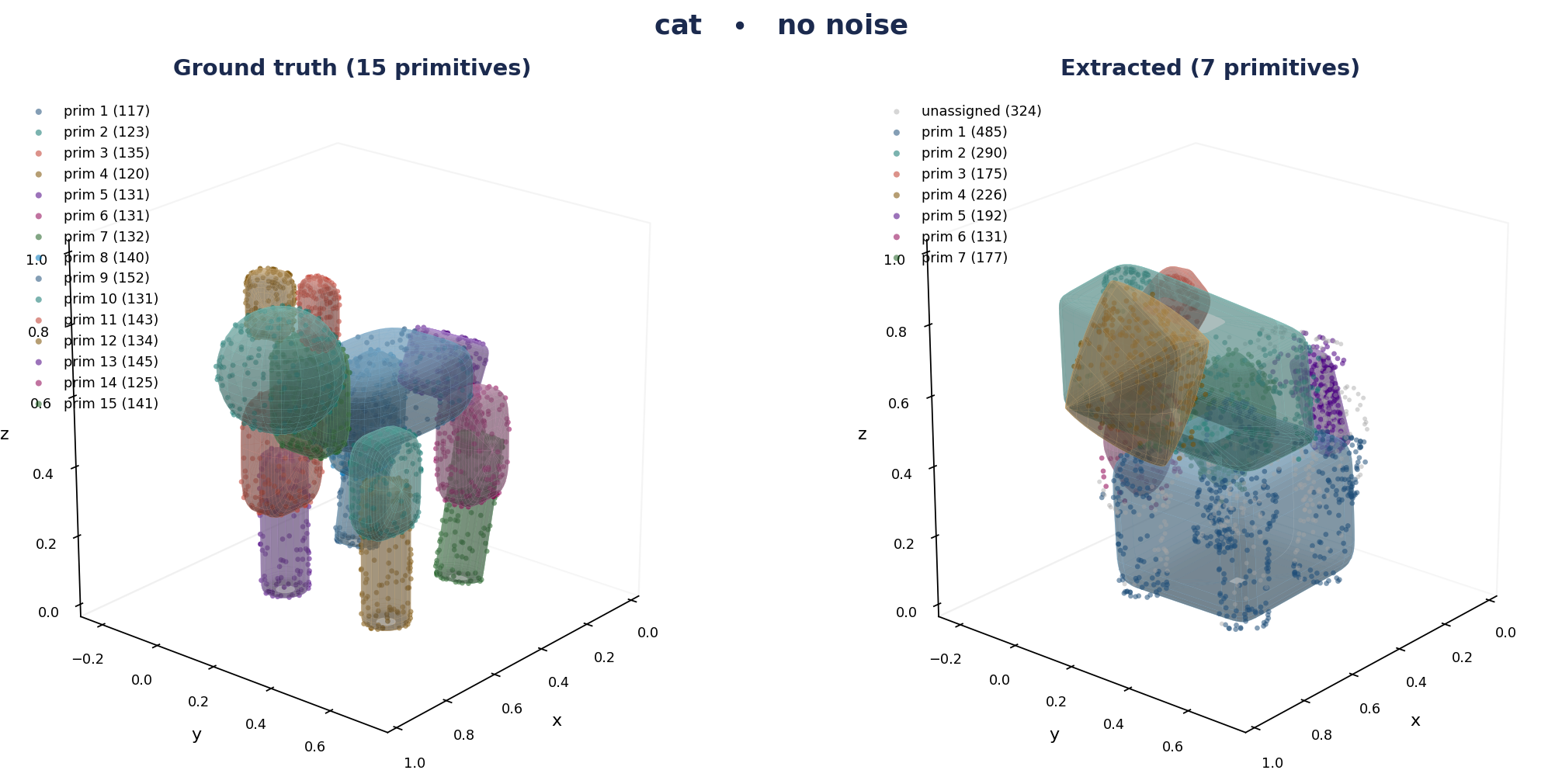
Ground-truth labels and surfaces on the left, our extracted primitives on the right. The pipeline runs with one parameter set across every scene below.

−40%

mean Chamfer distance
4.1 → 2.5 ×10⁻³

88.8%

mean inlier coverage
on 9 / 10 meshes

94%+

single-model recall
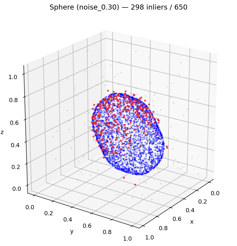
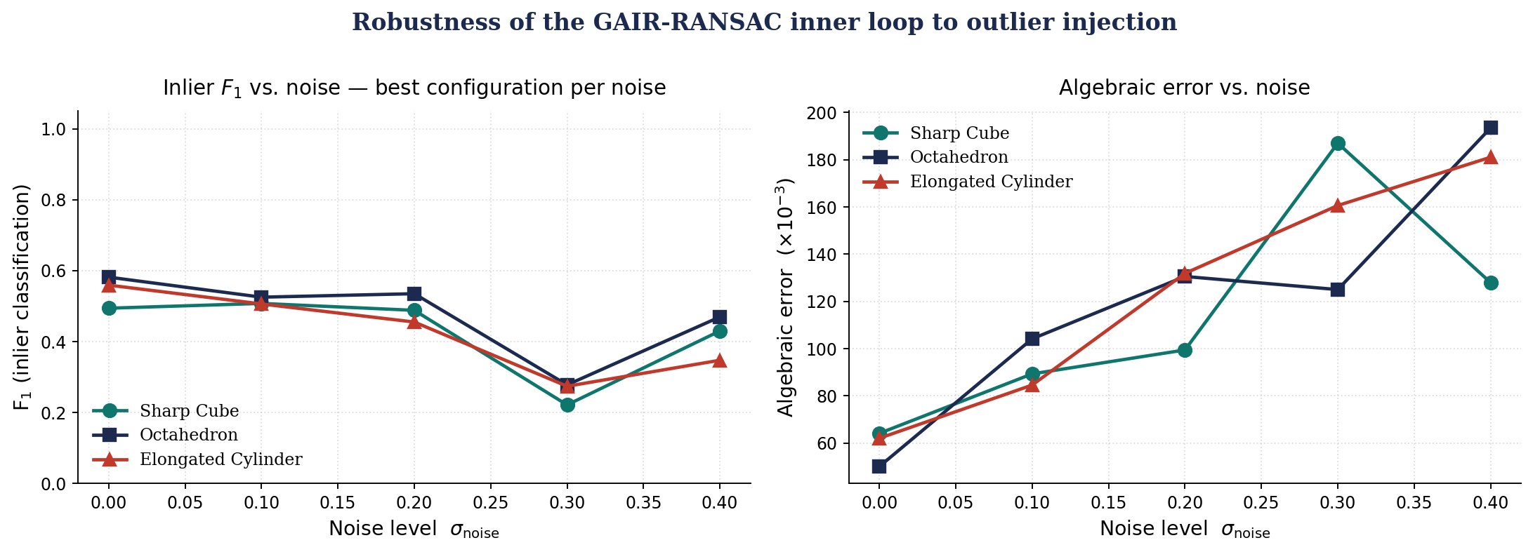
up to σ = 0.30 noise

Tuning the full pipeline meant searching $\sim\!15$ hyper-parameters, so a Cartesian grid was prohibitive. We ran a 9-stage greedy grid search (exactly 126 configurations) over the 10 Thingi10K probe meshes, optimising the average symmetric Chamfer distance and carrying the best values forward at each stage. Two stages dominated: swapping in the radial residual cut Chamfer by 27% at fixed coverage, and tuning the MSS normal-angle threshold to $75^\circ$ — which stops curved patches from fragmenting — gave a further 32% drop. The final defaults: radial residual, $\lambda_w=0.3$, $f_{\text{scale}}=0.5$, soft-L1 loss, $\varepsilon=0.08$, $\tau_C=0.5$, $\tilde\tau_C=0.85$, $n_{\text{at}}=75^\circ$, $\lambda_{\text{size}}=0.05$.

Per-shape results — final configuration on Thingi10K

Shape ID	Chamfer (×10⁻³)	Inlier ratio	# Primitives
1005276	2.91	0.857	3
131969	1.86	0.927	4
1344040	1.74	0.999	3
37384	1.92	0.821	3
39643	2.06	0.907	5
44102	2.86	0.725	1
488050	2.48	0.895	2
678267	2.34	0.963	2
90279	1.73	0.894	4
Mean	2.54	0.888	—

Remaining failure modes. Densely jointed scenes still force greedy "containment fits" across touching objects, tripping the coverage gate; and superquadrics are convex, so concave geometry needs several primitives. Both point to the same fix — replacing the greedy loop with a global multi-label graph cut, plus an MDL criterion to choose $\kappa$ automatically.

Pipeline overview — The full pipeline. Orange = new graph-side ingredients; green = post-extraction global refinement.

Radial vs algebraic residual — Why the radial residual matters: the algebraic residual diverges below ε = 0.3, hiding sharp shapes from the fitter.

Single sphere under 30% noise — A single sphere recovered under 30% outliers — radius estimated within ~1% of ground truth.

Multi-model random disjoint scene — Four free-form primitives in arbitrary poses — all recovered, with predicted clusters matching ground-truth instances.

Real STL mesh 131969 — Real Thingi10K mesh #131969 — four superquadrics capture the body plus three protrusions.

Real STL mesh 1344040 — Mushroom-like mesh #1344040 — cap, neck and body fit with no per-mesh tuning.

Cat scene decomposition — A multi-part "cat" scene decomposed into its primitive components.

F1 vs noise ablation — F₁ score degrades gracefully up to σ = 0.30 across all five canonical shapes.

07 — Why it matters

Where robust primitive fitting pays off

Robotic grasping

A gripper plans far better against "a cylinder here, a box there" than against a raw point cloud. Superquadrics give collision-friendly, graspable volumes.

Reverse engineering / CAD

Turn a 3D scan of a part into a small set of editable parametric solids — the first step from scan to manufacturable model.

Scene understanding

Compact part-level abstractions are cheap to store, match and reason over for AR, mapping and simulation.

Sensor-grade robustness

Holding one parameter set from clean data to 30% noise means it survives real RealSense captures, not just synthetic benchmarks.

Built on GAIR-RANSAC — Ferraris, Leveni, Baieri, Maggioli, Melzi & Magri, Smalltalk on Graphics (STAG) 2025 — and the classic superquadric recovery of Solina & Bajcsy (PAMI 1990).

Drag to explore the actual results

Why superquadrics, and why it's hard

Problem formulation

Six improvements over the paper

At a glance — paper vs. ours

Robust single-primitive fitting

Radial residual + volume penalty

The |F−1| inlier gate

Local-K sampling + PCA pose

Adaptive normal-coherency cut

Sequential multi-model extraction

Density-based pre-filter

Chamfer + coverage gates

Competitive reassignment + fission

From synthetic stress tests to real meshes

Per-shape results — final configuration on Thingi10K

Where robust primitive fitting pays off

Robotic grasping

Reverse engineering / CAD

Scene understanding

Sensor-grade robustness

The `|F−1|` inlier gate